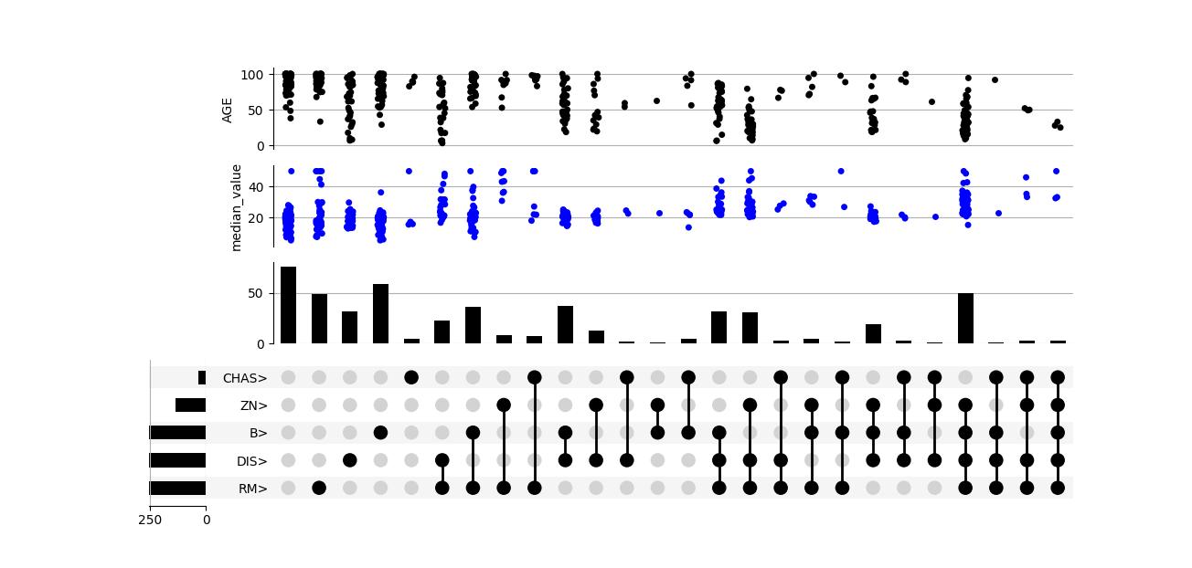
Above-average features in Boston

Explore above-average neighborhood characteristics in the Boston dataset.

Here we take some features correlated with house price, and look at the distribution of median house price when each of these features is above average.

The most correlated features are:

ZN

proportion of residential land zoned for lots over 25,000 sq.ft.

CHAS

Charles River dummy variable (= 1 if tract bounds river; 0 otherwise)

RM

average number of rooms per dwelling

DIS

weighted distances to five Boston employment centres

B

1000(Bk - 0.63)^2 where Bk is the proportion of blacks by town

This kind of dataset analysis may not be a practical use of UpSet, but helps to illustrate the UpSet.add_catplot() feature.

import pandas as pd
from sklearn.datasets import load_boston
from matplotlib import pyplot as plt
from upsetplot import UpSet

# Load the dataset into a DataFrame
boston = load_boston()
boston_df = pd.DataFrame(boston.data, columns=boston.feature_names)

# Get five features most correlated with median house value
correls = boston_df.corrwith(pd.Series(boston.target),
                             method='spearman').sort_values()
top_features = correls.index[-5:]

# Get a binary indicator of whether each top feature is above average
boston_above_avg = boston_df > boston_df.median(axis=0)
boston_above_avg = boston_above_avg[top_features]
boston_above_avg = boston_above_avg.rename(columns=lambda x: x + '>')

# Make this indicator mask an index of boston_df
boston_df = pd.concat([boston_df, boston_above_avg],
                      axis=1)
boston_df = boston_df.set_index(list(boston_above_avg.columns))

# Also give us access to the target (median house value)
boston_df = boston_df.assign(median_value=boston.target)

# UpSet plot it!
upset = UpSet(boston_df, sum_over=False, intersection_plot_elements=3)
upset.add_catplot(value='median_value', kind='strip', color='blue')
upset.add_catplot(value='AGE', kind='strip', color='black')
upset.plot()
plt.show()